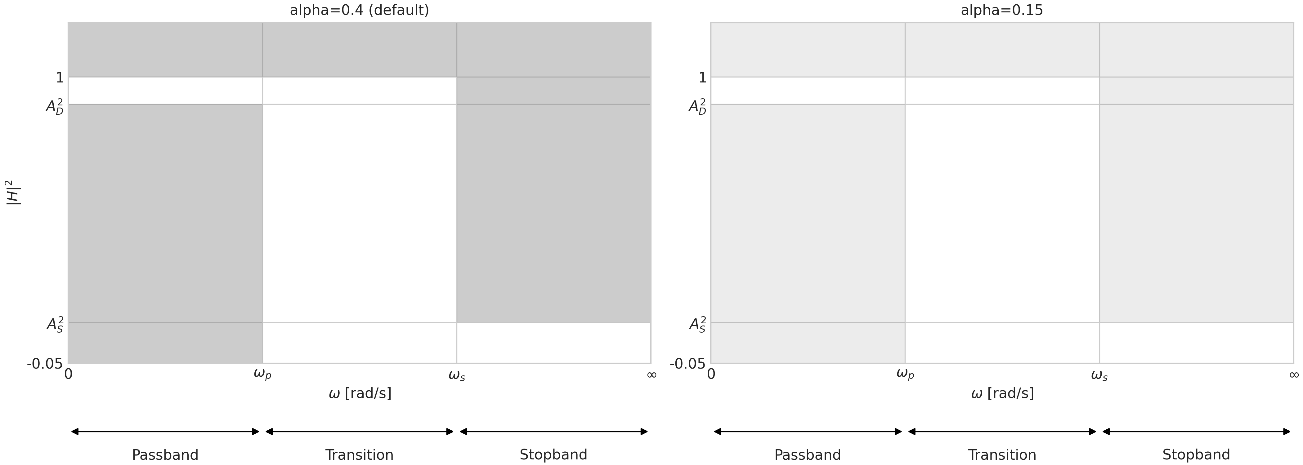
Plot Filter Tolerance

sysplot.plot_filter_tolerance() shades the forbidden regions of a filter power specification on an existing axes. Passband, stopband, and transition bands are defined as a list of dicts. The alpha parameter controls the shade opacity and defaults to filter_tolerance_alpha.

import matplotlib.pyplot as plt
import sysplot as ssp

ssp.apply_config()

A_pass = 0.9  # lower passband power bound (A_D\u00b2)
A_stop = 0.1  # upper stopband power bound (A_S\u00b2)
w_p = 1.0  # passband edge [rad/s]
w_s = 2.0  # stopband edge [rad/s]
w_max = 3.0

bands = [
    {
        "type": "pass",
        "w0": 0.0,
        "w1": w_p,
        "label": "Passband",
        "w0_label": r"$0$",
        "w1_label": r"$\omega_p$",
    },
    {
        "type": "transition",
        "w0": w_p,
        "w1": w_s,
        "label": "Transition",
        "w0_label": r"$\omega_p$",
        "w1_label": r"$\omega_s$",
    },
    {
        "type": "stop",
        "w0": w_s,
        "w1": w_max,
        "label": "Stopband",
        "w0_label": r"$\omega_s$",
        "w1_label": r"$\infty$",
    },
]

fig, axes = plt.subplots(1, 2, figsize=ssp.get_figsize(ncols=2))

# Default alpha (from SysplotConfig)
ax = axes[0]
ax.set_ylim(-0.05, 1.2)
ssp.plot_filter_tolerance(ax=ax, bands=bands, A_pass=A_pass, A_stop=A_stop, w_max=w_max)
ax.set(
    title=f"alpha={ssp.get_config().filter_tolerance_alpha} (default)",
    xlabel=r"$\omega$ [rad/s]",
    ylabel=r"$|H|^2$",
)

# Custom alpha
ax = axes[1]
ax.set_ylim(-0.05, 1.2)
ssp.plot_filter_tolerance(
    ax=ax, bands=bands, A_pass=A_pass, A_stop=A_stop, w_max=w_max, alpha=0.15
)
ax.set(title="alpha=0.15", xlabel=r"$\omega$ [rad/s]")

plt.show()