Quick Start Example

Covers the four main sysplot plot types applied to a second-order transfer function:

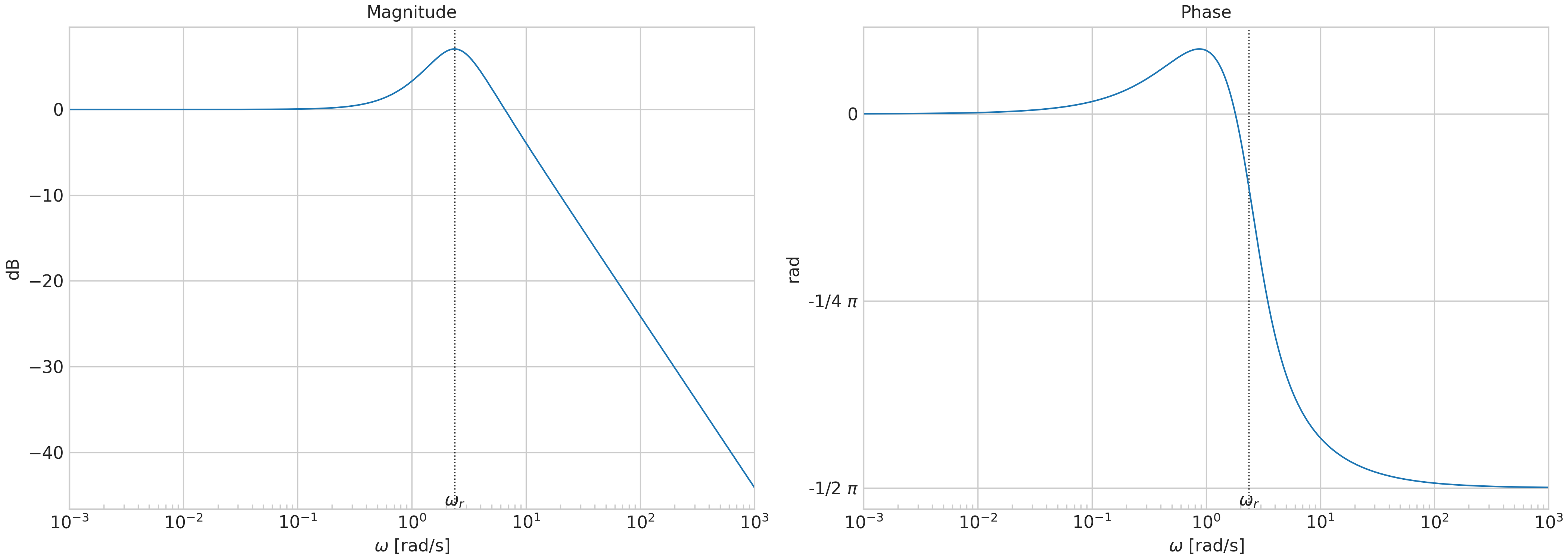
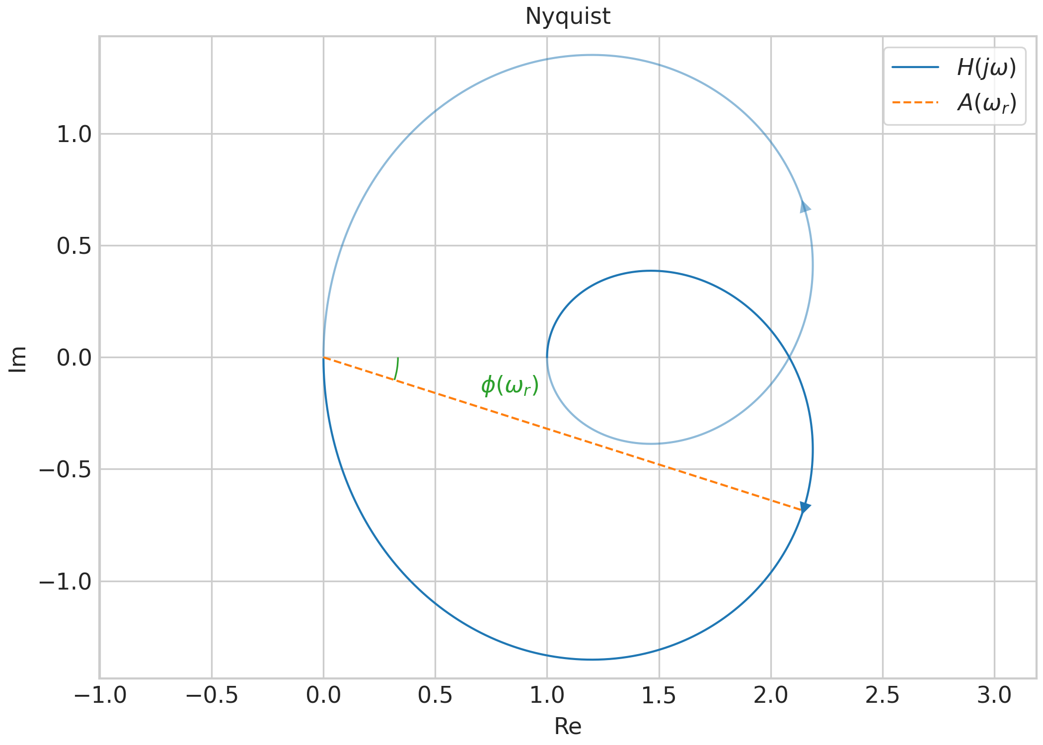
• Bode diagram — magnitude (dB) and phase (rad) vs. frequency with a custom resonance-frequency tick, using sysplot.plot_bode() and sysplot.add_tick_line().

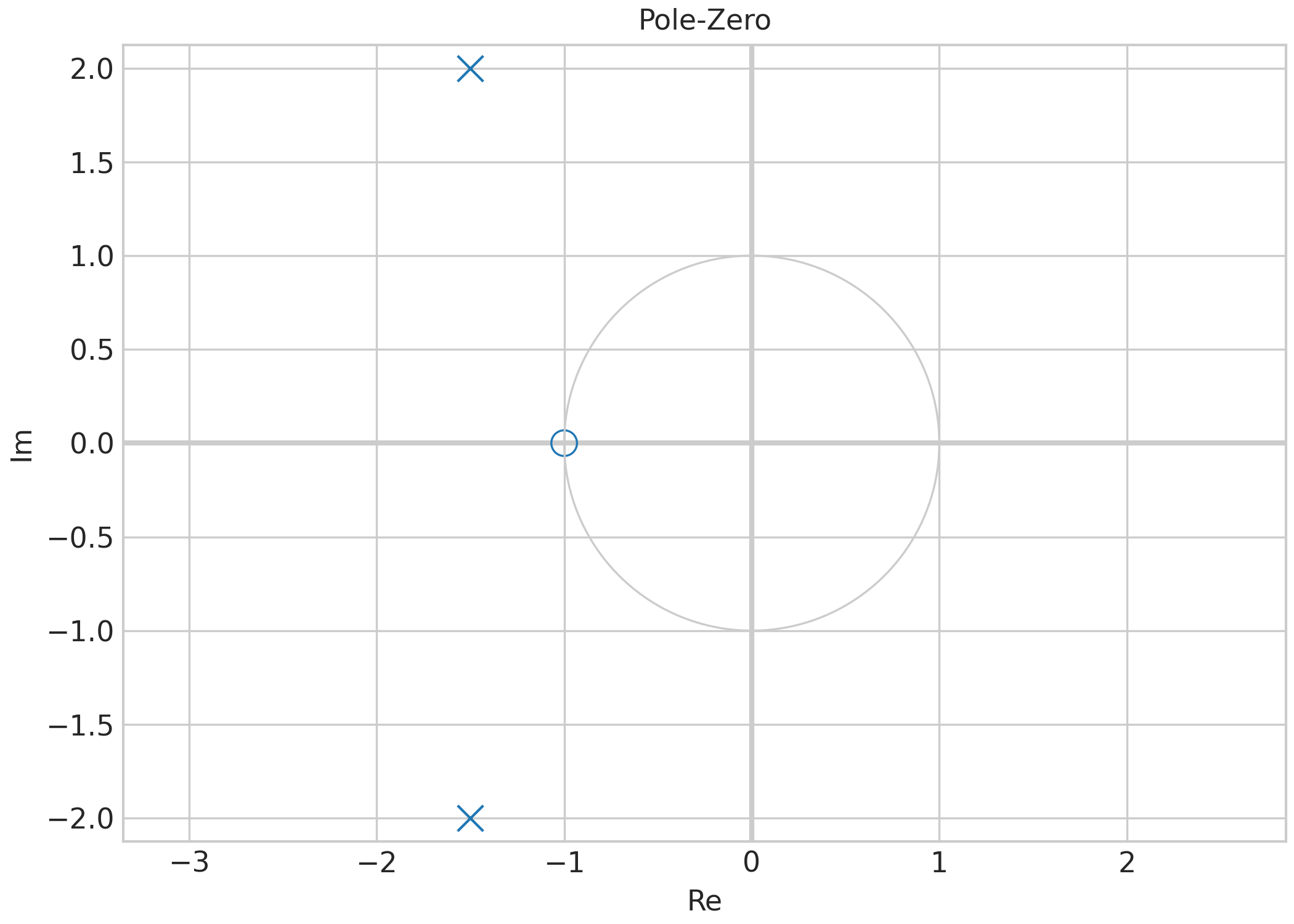
• Nyquist diagram — complex frequency response with direction arrow and angle annotation, using sysplot.plot_nyquist() and sysplot.plot_angle().

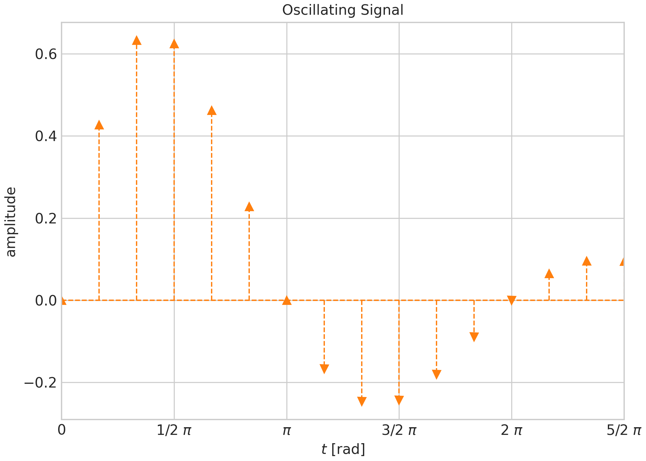
• Pole-zero map — poles, zeros, and unit circle overlaid on emphasised coordinate axes, using sysplot.plot_poles_zeros() and sysplot.plot_unit_circle().

• Stem plot — sampled damped sinusoid with outward-flipping markers, using sysplot.plot_stem().

• 
• 
• 
• 

import numpy as np
import matplotlib.pyplot as plt
import control as ctrl
import sysplot as ssp

# Apply sysplot default configuration
ssp.apply_config()


# =============================================================================
# Define Transfer Function
# =============================================================================

# Second-order system with zero: H(s) = ωₙ²(s + z) / (s² + 2ζωₙs + ωₙ²)
omega_n = 2.5  # natural frequency [rad/s]
zeta = 0.6  # damping ratio (< 1 for underdamped, gives resonance peak)
z = 1.0  # zero location at s = -1

system = ctrl.TransferFunction(
    [omega_n**2, omega_n**2 * z], [1, 2 * zeta * omega_n, omega_n**2]
)


# =============================================================================
# 1. Bode Plot
# =============================================================================

# Compute frequency response
omega = np.logspace(-3, 3, 4000)
mag, phase, _ = ctrl.frequency_response(system, omega)

# Create Bode diagram
fig, axes = plt.subplots(1, 2, figsize=ssp.get_figsize(1, 2), sharex=True)
ssp.plot_bode(
    mag,
    phase,
    omega,
    axes=axes,
    minor_ticks=True,
    mag_to_dB=True,
    x_to_log=True,
    tick_numerator=1,
    tick_denominator=4,
)

# Add custom tick at resonance frequency (peak magnitude)
omega_peak = omega[np.argmax(mag)]
ssp.add_tick_line(axis=axes[0].xaxis, value=omega_peak, label=r"$\omega_r$")
ssp.add_tick_line(axis=axes[1].xaxis, value=omega_peak, label=r"$\omega_r$")

axes[0].set(title="Magnitude", xlabel=r"$\omega$ [rad/s]", ylabel="dB")
axes[1].set(title="Phase", xlabel=r"$\omega$ [rad/s]", ylabel="rad")


# =============================================================================
# 2. Nyquist Plot
# =============================================================================

# Convert to complex frequency response
H = mag * np.exp(1j * phase)

fig, ax = plt.subplots()
ssp.plot_nyquist(
    real=np.real(H),
    imag=np.imag(H),
    mirror=True,  # show complex conjugate
    arrow_position=0.4,  # arrow at 40% of arc length
    label=r"$H(j\omega)$",
)

# show angle at length at peak magnitude
idx = np.argwhere(omega == omega_peak)[0][0]
p1 = (np.real(H[idx]), np.imag(H[idx]))
p2 = (1.0, 0.0)  # reference along +Re axis
plt.plot(*zip((0, 0), p1), label=r"$A(\omega_r)$", **ssp.get_style(index=1))
ssp.plot_angle(
    center=(0.0, 0.0),
    point1=p1,
    point2=p2,
    text=r"$\phi(\omega_r)$",
    size=300,
    color=ssp.get_style(index=2)["color"],  # get next color in the style cycler
)

ax.legend()
ax.set(title="Nyquist", xlabel="Re", ylabel="Im")


# =============================================================================
# 3. Pole-Zero Plot
# =============================================================================

poles = ctrl.poles(system)
zeros = ctrl.zeros(system)

fig, ax = plt.subplots()
ssp.emphasize_coord_lines(fig)
ssp.plot_poles_zeros(poles=poles, zeros=zeros, show_origin=True)
ssp.plot_unit_circle(ax=ax, origin=(0, 0))

ax.set(title="Pole-Zero", xlabel="Re", ylabel="Im")


# =============================================================================
# 4. Stem Plot with Automatic Marker Flipping
# =============================================================================

# Generate damped sinusoid with zero-crossings
t_sample = np.linspace(0, 5 / 2 * np.pi, 16)
signal = np.exp(-0.3 * t_sample) * np.sin(t_sample)

fig, ax = plt.subplots()
ssp.plot_stem(
    x=t_sample,
    y=signal,
    bottom=0,
    marker="^",
    directional_markers=True,  # markers flip when crossing baseline
    continous_baseline=True,
    **ssp.get_style(index=1),
)

# Show x-axis in multiples of π
ssp.set_major_ticks(
    label=r"$\pi$", unit=np.pi, numerator=1, denominator=2, axis=ax.xaxis
)

ax.set(title="Oscillating Signal", xlabel=r"$t$ [rad]", ylabel="amplitude")

plt.show()