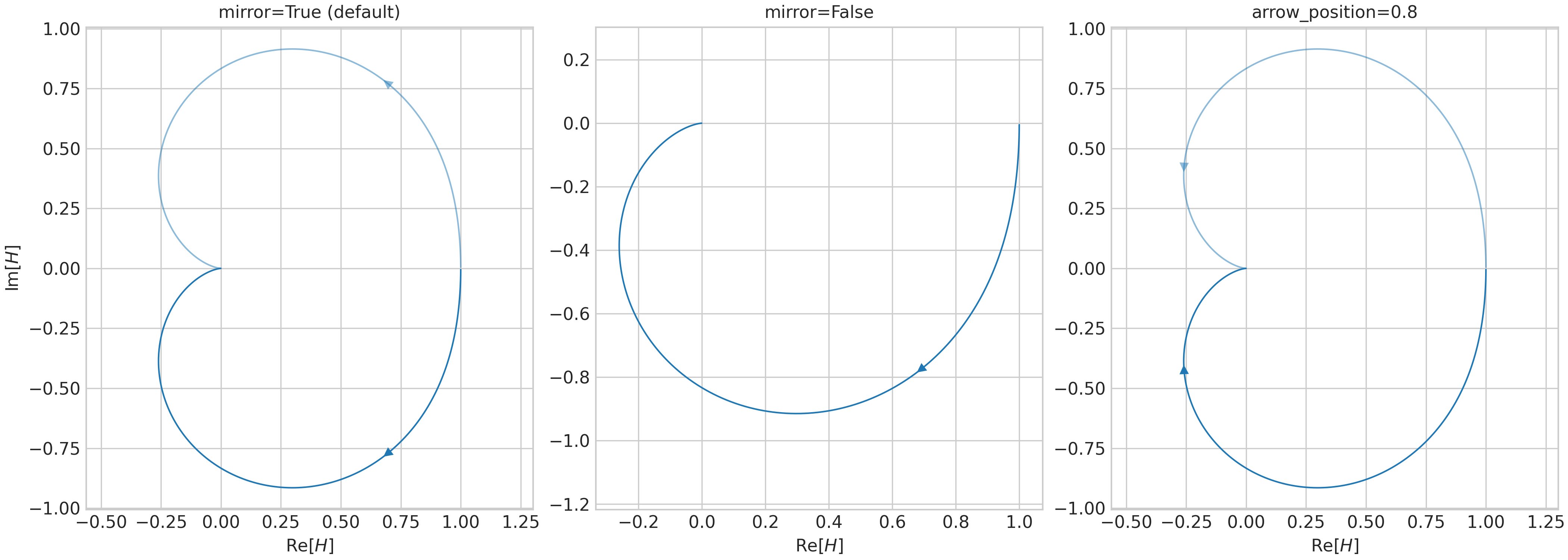
Plot Nyquist

sysplot.plot_nyquist() draws the Nyquist diagram of a frequency response in the complex plane. A directional arrow marks the direction of increasing frequency. The complex conjugate (mirror) curve is shown at reduced opacity, controlled by alpha. The arrow position along the curve arc length is set by arrow_position.

import numpy as np
import matplotlib.pyplot as plt
import control as ctrl
import sysplot as ssp

ssp.apply_config()

system = ctrl.tf([6.25], [1, 3, 6.25])
omega = np.logspace(-2, 2, 1000)
mag, phase, _ = ctrl.frequency_response(system, omega)
real = mag * np.cos(phase)
imag = mag * np.sin(phase)

fig, axes = plt.subplots(1, 3, figsize=ssp.get_figsize(ncols=3))

# Default: mirror shown at half opacity, arrow at 33 % arc length
ssp.plot_nyquist(real, imag, ax=axes[0])
axes[0].set(title="mirror=True (default)", xlabel=r"Re[$H$]", ylabel=r"Im[$H$]")

# No mirror curve
ssp.plot_nyquist(real, imag, ax=axes[1], mirror=False)
axes[1].set(title="mirror=False", xlabel=r"Re[$H$]")

# Arrow placed later along the curve
ssp.plot_nyquist(real, imag, ax=axes[2], arrow_position=0.8)
axes[2].set(title="arrow_position=0.8", xlabel=r"Re[$H$]")

plt.show()